Urban LES intercomparison
Overview
Motivation for this project can be summed up in few key points
- Bright future: microscale turbulence resolving models – essential element of urban services and planning
- Aiding urban-canopy parameterizations in meso-scale & global-scale atmospheric models
- How good is LES in reproducing urban boundary layer?
- What approaches (numerics + physics) work best?
Participants
Currently there are 2 paticipant models:
- LES from RCC LMSU
Mixed dynamic subgrid closure + nesting Double-moment cloud microphysics & radiation (RRTM) modules Land surface coupling Atmospheric chemistry & aerosol transport CPU/GPU support via C/C++/MPI/OpenMP/CUDA
- Fluidity from Institute of Atmospheric Physics CAS
Basic Information for Fluidity: Numerics: Spatial discretisations: first-order and second-order Continuous Galerkin, Discontinuous Galerkin, Control Volume Temporal discretisation: first-order explicit, second-order semi-implicit and implicit Turbulence Package: Reynolds-Averaged Navier-Stokes (RANS) Modelling Generic length scale turbulence parameterization (based on two equations, for the transport of turbulent kinetic energy (TKE) and a generic second quantity) Standard k – ε Turbulence Model Large-Eddy Simulation (LES): Second-order dissipation model Fourth-order dissipation model Dynamic Smagorinsky model
to become a participant send an email to Andrey Debolskiy or Evgeny Mortikov
Stages
Idealized urban configurations
The preliminary setup follows JAS paper 1
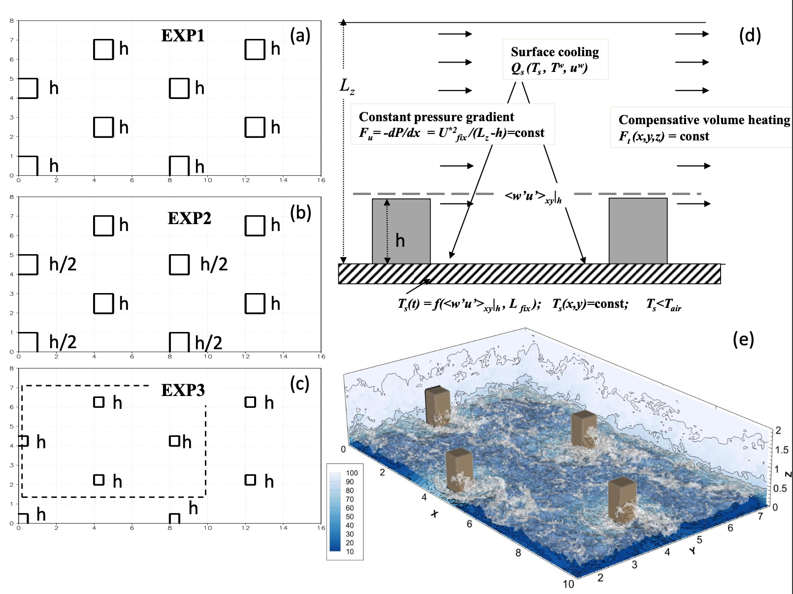
here is a scheme for the experiments

for testing non-stratified flow is considered. Here has detailed description of the idealized setup. Below is just a breif overview
- Domain:
length = 256 m, width = 128 m, height = 64.0 m; - Grid:
nx = 512; ny = 256; nz = 128, so that uniform resolution of 0.5m in any direction is achieved - Flow configuration: Open Channel flow with constant external pressure gradient of
dpdx = - phys.rho_ref * ustar_r^2 /(height - buildings_height), wherephys.rho_ref = 1.25 kg/m^3is reference air density,ustar_roof = 0.25is target dynamic velocity just above the building roofs . - Other fluid characteristics:
f = 0.0; # coriolis frequency [1/s] nu = 1.25 * 0.00001; # kinematic viscosity [m^2/s] xi = (1.0 / 0.7) * nu; # thermal diffusivity [m^2/s] rho_ref = 1.25; # reference density of air [kg/m^3] g = 9.81; # gravitational acceleration [m/s^2] Theta_ref = 283.15; # reference temperature [K] # --- no buoyancy beta = 0.0; # = g * thermal expansion coefficient = g / Theta_ref [m/(K*s^2)] - Integration model time: 2hours
- Buildings setup: surface dynamic and thermal roughness parameters
z0m = 0.01 m,z0h = z0m/10.0.building_height = 16 m. - Building configuration: EXP1
h = 16 # [m], building height patch_1 { type = "box"; xmin = 0.0; xmax = h; # patch dimensions ymin = 0.0; ymax = h; height = h; xperiod = 8.0 * h; # periodicity in -x yperiod = 4.0 * h; # periodicity in -y } patch_2 { type = "box"; # patch type: "box" || "hill" xmin = 4.0 * h ; xmax = 5.0 * h; # patch dimensions ymin = 2.0 * h; ymax = 3.0 * h; height = h; xperiod = 8.0 * h; # periodicity in -x yperiod = 4.0 * h; # periodicity in -y } - EXP2
h = 16 # [m], building height patch_1 { type = "box"; xmin = 0.0; xmax = h; # patch dimensions ymin = 0.0; ymax = h; height = h; xperiod = 8.0 * h; # periodicity in -x yperiod = 4.0 * h; # periodicity in -y } patch_2 { type = "box"; # patch type: "box" || "hill" xmin = 4.0 * h ; xmax = 5.0 * h; # patch dimensions ymin = 2.0 * h; ymax = 3.0 * h; height = h/2.0; xperiod = 8.0 * h; # periodicity in -x yperiod = 4.0 * h; # periodicity in -y } - EXP3
h = 16 # [m], building height
        patch_1 {
                type = "box";

                xmin = 0.0; xmax = h/2.0;   # patch dimensions
                ymin =  0.0; ymax = h/2.0;
                height = h;

                xperiod = 8.0 * h;                      #  periodicity in -x
                yperiod = 4.0 * h;                      #  periodicity in -y
        }
        patch_2 {
                type = "box";                   # patch type: "box" || "hill"

                xmin = 4.0 * h ; xmax = 4.5 * h;   # patch dimensions
                ymin =  2.0 * h; ymax = 2.5 * h;
                height = h;

                xperiod = 8.0 * h;                  # periodicity in -x
                yperiod = 4.0 * h;                  # periodicity in -y
        }
Stratified idealized urban cases
coming soon
Realistic urban developments
cooming soon
Outputs
for output see notebooks here
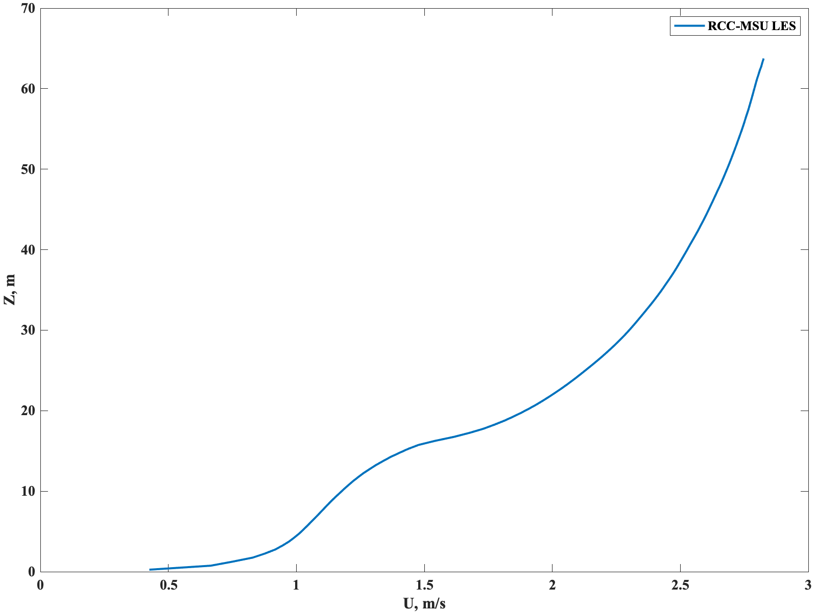
Example of output for EXP1
